
Over reading week, I got the chance to attend a workshop in gate-based quantum computing. This was a joint venture between UBC’s Quantum Matter Institute and industry partners 1QBit and Rigetti Computing.
As an computer engineering undergraduate, I had anticipated being in the minority at this workshop. So, what was I hoping to get out of it?
Well, for starters, I’ve a strong belief that one of the biggest benefits of a Bachelor’s degree is getting to explore random stuff for four years without the pressure of needing to produce a marketable product or publishable research. But, as well, I specifically wanted to answer the following questions:
- What exactly is quantum computing and why is it supposed to be so powerful?
- What is the current state of the art in quantum computing?
- How could quantum computing impact my future career as a software engineer, and on what time scale? (e.g., how soon should I throw out my RSA keys?)
- I am, as ever, still on the fence about pursuing an advanced degree in the future. Might I ever be interested in researching quantum computing?
With these questions in mind, this post summarises my main takeaways from the event.
Post scriptum: it got longer than intended. If you just want the short version, or would rather not see a little bit of linear algebra, skip to the end.
- How quantum computing works
- The quantum advantage
- The current state of quantum computing
- So, what can we do right now?
- Quantum supremacy
- Some questions
- Summary
How quantum computing works
The workshop began with an introduction to quantum computing for the uninitiated. As an uninitiated person, this was great.
Qubits
We began with a review of basic quantum mechanics: elementary particles have intrinsic angular momentum, called spin. Pick some arbitrary reference axis to measure along, and the particle will be aligned in either the spin up or spin down orientation, or somewhere in between.
This translates nicely to computing. Call the “up” orientation \(\lvert 0 \rangle\), and the “down” orientation \(\lvert 1 \rangle\) – now the particle kind of looks like it could be used to represent a bit. But quantum bits have some cool features that regular bits don’t have.
Superposition
If our classical bit is somewhere between 0 and 1, then we complain about transistor leakage and throw it away. But if we have a qubit that is between \(\lvert 0 \rangle\) and \(\lvert 1 \rangle\), it’s a feature, not a bug.
To express superposition, we write the qubit as a linear combination of the two “pure” states: \(\lvert \Psi \rangle = c_1 \lvert 0 \rangle + c_2 \lvert 1 \rangle\), where \(c_1\) and \(c_2\) are complex numbers (and the sum of their squared norms is 1).
More commonly, the term “basis” will be used to refer to these “pure” states. The equation that describes the superposition is also often called the “wave function” of the system.
We can alternatively use matrix notation and represent the qubit as a vector:
\[\lvert \Psi \rangle = \begin{pmatrix} c_1 \\ c_2 \end{pmatrix}\]So, a qubit contains within itself information about \(c_1\) and \(c_2\). The catch, however, is that as a programmer, you can’t access \(c_1\) or \(c_2\) directly – the only information you can extract from the qubit is whether it’s \(\lvert 0 \rangle\) or \(\lvert 1 \rangle\), and you do that by measuring it, whereupon you will get either \(\lvert 0 \rangle\) with probability \(\lvert c_1 \lvert ^2\), or \(\lvert 1 \rangle\) with probability \(\lvert c_2 \lvert^2\).
Since you have to get one of the states when you measure, it follows that \(\lvert c_1 \lvert ^2 + \lvert c_2 \lvert ^2 = 1\).
Also, once you measure it, all the information about \(c_1\) and \(c_2\) disappear from the qubit.
This is important enough to warrant repeating: you cannot extract information about \(c_1\), \(c_2\). 1
Entanglement
Another feature of qubits is that you can put more than one of them into an entangled state. In statistical terms, if two qubits are entangled, then the probabilities of measuring \(\lvert 0 \rangle\) or \(\lvert 1 \rangle\) for each qubit is no longer conditionally independent.
The Bell state is an example of a 2-qubit entanglement:
\[\lvert \Psi_1 \Psi_2 \rangle = \frac{1}{\sqrt{2}} \lvert 00 \rangle + \frac{1}{\sqrt{2}} \lvert 11 \rangle\]If you were to measure the two qubits, you would have a 50% chance of observing both qubits in state \(\lvert 0 \rangle\) and a 50% chance of observing both of them in state \(\lvert 1 \rangle\). You would have no chance of observing them in different states.
If two qubits are entangled, then there is a single wave function that describes both of them. They are not separably describable by two wave functions.
It follows that a qubit that is in a basis state can’t be entangled – it is always separable from the other qubits in the system.
Multiple qubits
We often want to entangle many qubits. But it would be very tedious to write out all their states using conditional probabilities. So, we do the same thing as for the single qubit: write the multi-qubit system as a weighted sum of the basis states.
It turns out that the basis of a multi-qubit system consists of every possible combination of the individual qubits’ basis states. So, for the 2-qubit system:
\[\lvert \Psi_1 \Psi_2 \rangle = c_1 \lvert 00 \rangle + c_2 \lvert 01 \rangle + c_3 \lvert 10 \rangle + c_4 \lvert 11 \rangle\]Or, as a vector:
\[\lvert \Psi_1 \Psi_2 \rangle = \begin{pmatrix}c_1 \\ c_2 \\ c_3 \\ c_4 \end{pmatrix}\]As before, \(c_1, c_2, c_3, c_4\) are complex numbers, and the sum of their squared norms is \(1\). If measured, this 2-qubit system would have a probability \(\lvert c_1 \lvert^2\) of being observed in state \(\lvert 00 \rangle\), a probability \(\lvert c_2 \lvert^2\) of being observed in state \(\lvert 01 \rangle\), \(\lvert c_3 \lvert^2\) for state \(\lvert 10 \rangle\), and \(\lvert c_4 \lvert^2\) for state \(\lvert 11 \rangle\).
A 3-qubit system is expressed as:
\[\lvert \Psi_1 \Psi_2 \Psi_3 \rangle = c_1 \lvert 000 \rangle + c_2 \lvert 001 \rangle + c_3 \lvert 010 \rangle + c_4 \lvert 011 \rangle + c_5 \lvert 100 \rangle + c_6 \lvert 101 \rangle + c_7 \lvert 110 \rangle + c_8 \lvert 111 \rangle\]Or, as a vector:
\[\lvert \Psi_1 \Psi_2 \Psi_2 \rangle = \begin{pmatrix} c_1 \\ c_2 \\ c_3 \\ c_4 \\ c_5 \\ c_6 \\ c_7 \\ c_8 \end{pmatrix}\]If measured, this system has a \(\lvert c_1 \lvert^2\) probability of being observed in state \(\lvert 000 \rangle\), a \(\lvert c_2 \lvert^2\) probability of… well, you get the point.
An \(n\)-qubit system has \(2^n\) basis states and is represented as a \(2^n \times 1\) vector. Every single sequence of qubits can be represented this way, but you need exponentially more space to represent it.
As with the 1-qubit system, you still cannot get any information about any \(c_i\) out of the system. Once you measure your \(n\)-qubit system, you will get one of the \(2^n\) basis states.
Also, as with the 1-qubit system, since you have to get one of the basis states when you measure, it follows that \(\sum_{i=1}^{2^n} \lvert c_i \lvert^2 = 1\).
Quantum gates
Classical computing has logic gates. So does quantum computing.
We can write quantum gates as truth tables, but it is convenient to think of them as matrices. Then applying a gate to a qubit is basically multiplying the gate by the qubit.
Single qubit gates
These operate on our single qubit, \(\lvert \Psi \rangle = (c_1, c_2)^T\). They will alter the values \(c_1, c_2\).
A particularly important single qubit gate is the Hadamard gate:
\[H = \frac{1}{\sqrt{2}}\begin{pmatrix}1 & 1 \\ 1 & -1 \end{pmatrix}\]Or, as a truth table:
| \(\lvert \Psi \rangle\) | \(H \lvert \Psi \rangle\) |
|---|---|
| \(\lvert 0 \rangle\) | \(\frac{1}{\sqrt{2}}(\lvert 0 \rangle + \lvert 1 \rangle)\) |
| \(\lvert 1 \rangle\) | \(\frac{1}{\sqrt{2}}(\lvert 0 \rangle - \lvert 1 \rangle)\) |
Ick. Matrices are so much simpler.
The Hadamard gate is important because it creates a superposition out of a boring basis qubit. Many quantum algorithms start with Hadamarding everything in sight, because then you can do something interesting with it.
Two-qubit gates
These operate on 2 qubits at once. Which, since a 2-qubit system is a \(4 \times 1\) matrix, means that the gate is a \(4 \times 4\) matrix.
You can turn any two 1-qubit gates into a 2-qubit gate by taking the tensor product of their matrices. For example:
\[H \otimes I = \begin{pmatrix}\frac{1}{\sqrt{2}} & 0 & \frac{1}{\sqrt{2}} & 0 \\ 0 & \frac{1}{\sqrt{2}} & 0 & \frac{1}{\sqrt{2}} \\ \frac{1}{\sqrt{2}} & 0 & \frac{1}{\sqrt{2}} & 0 \\ 0 & -\frac{1}{\sqrt{2}} & 0 & -\frac{1}{\sqrt{2}} \end{pmatrix}\]Applying this gate to a 2-qubit system has the same effect as applying Hadamard to the first qubit, and leaving the second one alone.
A particularly important 2-qubit gate is the controlled-NOT, or CNOT gate:
\[CNOT = \begin{pmatrix}1 & 0 & 0 & 0 \\ 0 & 1 & 0 & 0 \\ 0 & 0 & 0 & 1 \\ 0 & 0 & 1 & 0 \end{pmatrix}\]In classical terms, the CNOT flips qubit 2 if and only if qubit 1 is set. But, since qubits are rarely “set” or “not set”, what the CNOT actually does is swap the likelihoods of \(\lvert 10 \rangle\) and \(\lvert 11 \rangle\), while leaving \(\lvert 00 \rangle\) and \(\lvert 01 \rangle\) untouched.
The CNOT is super important because it entangles qubits. Recall the Bell state briefly shown earlier. It turns out that it can be created from two boring basis qubits by using a Hadamard on one of the qubits, followed by a CNOT gate on both of them:
\[\lvert \Psi_1 \Psi_2 \rangle = \begin{pmatrix}1 \\ 0 \\ 0 \\ 0 \end{pmatrix} \quad \text{initial state, } \lvert 00 \rangle\] \[\begin{pmatrix}\frac{1}{\sqrt{2}} & 0 & \frac{1}{\sqrt{2}} & 0 \\ 0 & \frac{1}{\sqrt{2}} & 0 & \frac{1}{\sqrt{2}} \\ \frac{1}{\sqrt{2}} & 0 & \frac{1}{\sqrt{2}} & 0 \\ 0 & -\frac{1}{\sqrt{2}} & 0 & -\frac{1}{\sqrt{2}} \end{pmatrix} \begin{pmatrix}1 \\ 0 \\ 0 \\ 0 \end{pmatrix} = \begin{pmatrix} \frac{1}{\sqrt{2}} \\ 0 \\ \frac{1}{\sqrt{2}} \\ 0 \end{pmatrix} \quad \text{Hadamard qubit 1}\] \[\begin{pmatrix}1 & 0 & 0 & 0 \\ 0 & 1 & 0 & 0 \\ 0 & 0 & 0 & 1 \\ 0 & 0 & 1 & 0 \end{pmatrix} \begin{pmatrix} \frac{1}{\sqrt{2}} \\ 0 \\ \frac{1}{\sqrt{2}} \\ 0 \end{pmatrix} = \begin{pmatrix} \frac{1}{\sqrt{2}} \\ 0 \\ 0 \\ \frac{1}{\sqrt{2}} \end{pmatrix} \quad \text{Bell state}\]You can then entangle more qubits by applying more CNOTs.
There are also 3-qubit gates. And, in theory, you can have more complicated gates that operate on many qubits, but it’s unnecessary because….
Universal quantum gates
In classical computing, the NAND gate is a universal logic gate – that is, any possible operation on a classical computer can be reduced to NAND gates.
Similarly, in quantum computing, there are sets of universal logic gates to which any possible operation can be reduced. The most popular of these sets consist of the Hadamard, the CNOT, and the phase shift (\(R_\phi\)) gate.
If you have access to these three gates, you can make a quantum turing machine.
The quantum advantage
(in theory)
Classically, as we’ve seen above, an \(n\)-qubit system requires \(2^n\) space to even be represented. Operating on this system requires multiplying it by a \(2^n \times 2^n\) matrix. With a classical computer, this takes \(O(2^{3n})\) time. So, quantum operations can be extremely powerful.
They’re still limited to being linear operations, which is disappointing because getting rid of that limitation would let us do some really crazy stuff.
There is a gotcha: even though quantum operations could offer exponential speedups, and even though qubits appear to contain enormously more information than classical bits, you are very limited in what information you can get out of them.
An \(n\)-qubit system can be in some arbitrary superposition of \(2^n\) independent states, but once you measure it, you only get one of the \(2^n\) states in the readout. For the 2-qubit system, for example, your readout will be one of \(\vert 00 \rangle, \vert 01 \rangle, \vert 10 \rangle, \vert 11 \rangle\).
This is a bit of a mind warp to think about, but a qubit stores exactly the same quantity of information as a bit, even though it appears like they store more. If you read 2 bits out, you will also get one of \(\{ 00, 01, 10, 11 \}\).
The other thing to remember is that, before you read the 2 qubits, they were in some superposition \(c_1 \lvert 00 \rangle + c_2 \lvert 01 \rangle + c_3 \lvert 10 \rangle + c_4 \lvert 11 \rangle\), and which one of those you actually ended up getting is probabilistic based on \(c_1, c_2, c_3, c_4\). If you could measure the same qubits again (you can’t), you might get a different value.
Quantum algorithms
If you have qubits and gates, then putting a lot of qubits into a \(2^n\) superposition is very easy. But what you want is not to have a slop of superposed states – that makes for nice popular science articles (“you get to try all the paths at once!”), but doesn’t make for very useful computing, because when you measure the qubits you’ll just get some random state out.
The goal of a quantum algorithm is to create a final wave function that has a high probability of yielding the correct measurement for your given problem.
Designing an algorithm that can do this, for some problem that you’re interested in solving, is extremely difficult. Here are a few that have been created:
- Deutsch-Jozsa algorithm: determine whether an unknown “oracle” outputs a balanced or constant function using 1 test. Famous for being a first demonstration of where quantum computing could be superior to classical computing, but hard to think of real world applications for.
- Grover’s algorithm: find an element in an unordered input in \(O(\sqrt{n})\) time.
- Quantum phase estimation: given a matrix and an eigenvector for that matrix, find (an approximation) of its eigenvalue.
- Shor’s algorithm (of pop culture “it’s gonna break encryption!” fame): find prime factors exponentially faster than the best classical method.
Not all problems lend themselves easily to having unwanted states neatly cancel each other. All of the algorithms mentioned above exploit some fact about the problem that they’re solving, that makes them particularly well suited to a quantum solution.
For example, Shor’s algorithm exploits the periodicity of the remainders of the powers of an integer when divided by a product of two primes to create a superposition in which the wrong answers destructively interfere. [more detailed explanation]
Grover’s algorithm requires an oracle that can identify the correct result, and uses it to amplify the correct basis until its probability is sufficiently high. [more detailed explanation]
Research into quantum algorithms is very active right now! If you think looking for cool tricks like these sounds like something you’d enjoy devoting a good chunk of your life to, then you were definitely born in the right era.
The current state of quantum computing
We don’t have a large trove of useful quantum algorithms yet. In fact, the question of how useful quantum algorithms might ever get is still an open question – for example, a lot of people who seem to know what they’re talking about are pretty sure that quantum computers can’t solve NP problems in polynomial time.2 This was disappointing to learn, since pop science had told me that quantum computers were going to make travelling salesmen really happy.
Nevertheless, what quantum algorithms we do have are still pretty useful. For example, during the workshop, it was mentioned that a 1000-qubit universal quantum computer could break RSA in a day, compared to months for the current fastest supercomputers.3
So, what’s holding us back from this 1000-qubit universal quantum computer?
Um, well… basically it’s really hard to make these things. There are many factors in evaluating the quality of a quantum computer. Here are a few important ones:
Gate fidelity
Current generation CNOT gates have errors in the range of 5-10%. This is not completely unusable, but the more useful algorithms require using a lot of gates. Current generation gates are effectively unusable for these algorithms.
Single qubit gates are better, but still have room for improvement.
Coherence time
Qubits need to remain coherent throughout the duration of the computation. This is difficult to do, because for qubits to remain coherent, they must be perfectly isolated from their surroundings.
Any interaction with the environment will also cause the system to decohere into a classical probability distribution of basis states. This is sometimes described as “losing information” to the environment. This will introduce errors into your computation, because classical systems can’t do cool stuff like interfere with itself to amplify the desired state.
I’m still not convinced that I really grok the concept of decoherence, so I’ll just leave it like this: decoherence bad. Break quantum algorithms. Make error.
Currently, the best coherence times for qubits are in the range of seconds.
Quantum error correction
This seems like as good a time as any to introduce quantum error correction.
We are already well versed in error correction codes from classical computing, where bit flips are accepted as a fact of life. But error correction is a good deal trickier in quantum computing due to the fact that you can’t read or copy qubits.
The good news is that all hope is not lost. The field of quantum error correction is really, really interesting, because it tries to solve the problem of how to detect and correct an error in a qubit that you’re not allowed to measure. I could probably spend way too much time deep diving into it. But the key takeaways are:
- quantum error correction is possible and could, in theory, be used to create perfect qubits that are immune to decoherence and other noise
- this requires that the qubits have fewer than 1 error per 1000 (or so) gates, which we’re nowhere near
- there is an overhead: it takes 7 qubits to create 1 fault-tolerant qubit
- there is also a computational overhead, as quantum gates are needed to do the correction
- cheaper codes exist, but no proven fault-tolerance threshold yet exists for them, so for now we’re stuck with the 7:1 overhead
Connectivity
We would like to create really large superpositions.
It is much easier to create superpositions between nearby qubits, but in an ideal world we might also like to create superpositions between arbitrary qubits regardless of how they are laid out.
Connecting qubits is further complicated by the fact that, the more connectivity there is, the more chances there are for qubits to accidentally interact with the environment. This is why the best decoherence times are always measured on single, isolated qubits.
So, what can we do right now?
Well, we can’t realistically use any of the cool quantum algorithms, because qubits are too fragile and gates are too wonky to produce anything useful. But suppose you’re an eager undergraduate (or grad student, whatever) jonesing to get your hands on something quantum-y that can do computations. This is what you can do.
Simulators
We got a hands-on tour of Rigetti’s quantum simulator. I teleported a qubit!
Because it takes exponential space to store the state vectors and matrices, simulators are currently capped at ~20 qubits, depending on how much RAM your computer has. But they are a nice way to try out some basic quantum computing algorithms.
Noisy intermediate-scale quantum computers (NISQ)
What quantum computers do exist in the real world currently max out at around 50 qubits. They have too low gate fidelity to achieve fault-tolerance, and probably don’t want to spare any qubits for error correction anyway, so they are noisy.
We will likely have to put up with NISQ for quite a while, but a lot of research effort is being put toward developing better qubits, better gates, and implement fault tolerance, in academia as well as in industry.
Because of their high error rates, NISQs are not well suited to algorithms like Shor’s, which require a large number of gates. So, until fault tolerant quantum computers (FTQs?) come along, we’re largely stuck with….
Hybrid quantum-classical algorithms
These algorithms use a mixture of classical and quantum computation. They are designed to minimise the number of gates and the number of qubits.
Hybrid quantum-classical algorithms are well suited to optimization problems where the cost function of the solution can be encoded as a Hamiltonian, ideally one that can be computed using very few gates. Then, as with classical optimization, the goal is to search for the solution with the lowest cost.
We learned about a few different hybrid algorithms: variational quantum eigensolver (VQE), quantum approximate optimization algorithm (QAOA), and the cutely named “vanQver.” At a high level, they all boil down to the same thing:
- Figure out how to represent your problem using a small set of parameters
- Construct a Hamiltonian that represents your objective function
- Construct an initial parameter “guess”
- Encode the Hamiltonian into a quantum circuit; run it with the guess and measure the output
- Repeat step 4 many times to get an estimate of the expectation value of the output, which is in turn an estimate of the “best” value for that particular set of parameters
- Modify the guess to try and improve the outcome
- Repeat steps 4 to 6 until you’re pretty sure you’ve found the best possible outcome
- Output the parameters that produced this best outcome
Steps 1 and 2 are done by a human expert. Step 2, in particular, is non-trivial. I got the impression that a pretty big portion of 1Qbit’s work is doing exactly these two steps.
Step 4 is done on the quantum computer.
Steps 3 and 5-8 are done on a classical computer. In brief, you’re running a classical optimization routine on the classical computer, and the goal of the optimization routine is to minimize (or maximize) the output of the quantum computer, which the classical computer treats as a black box.
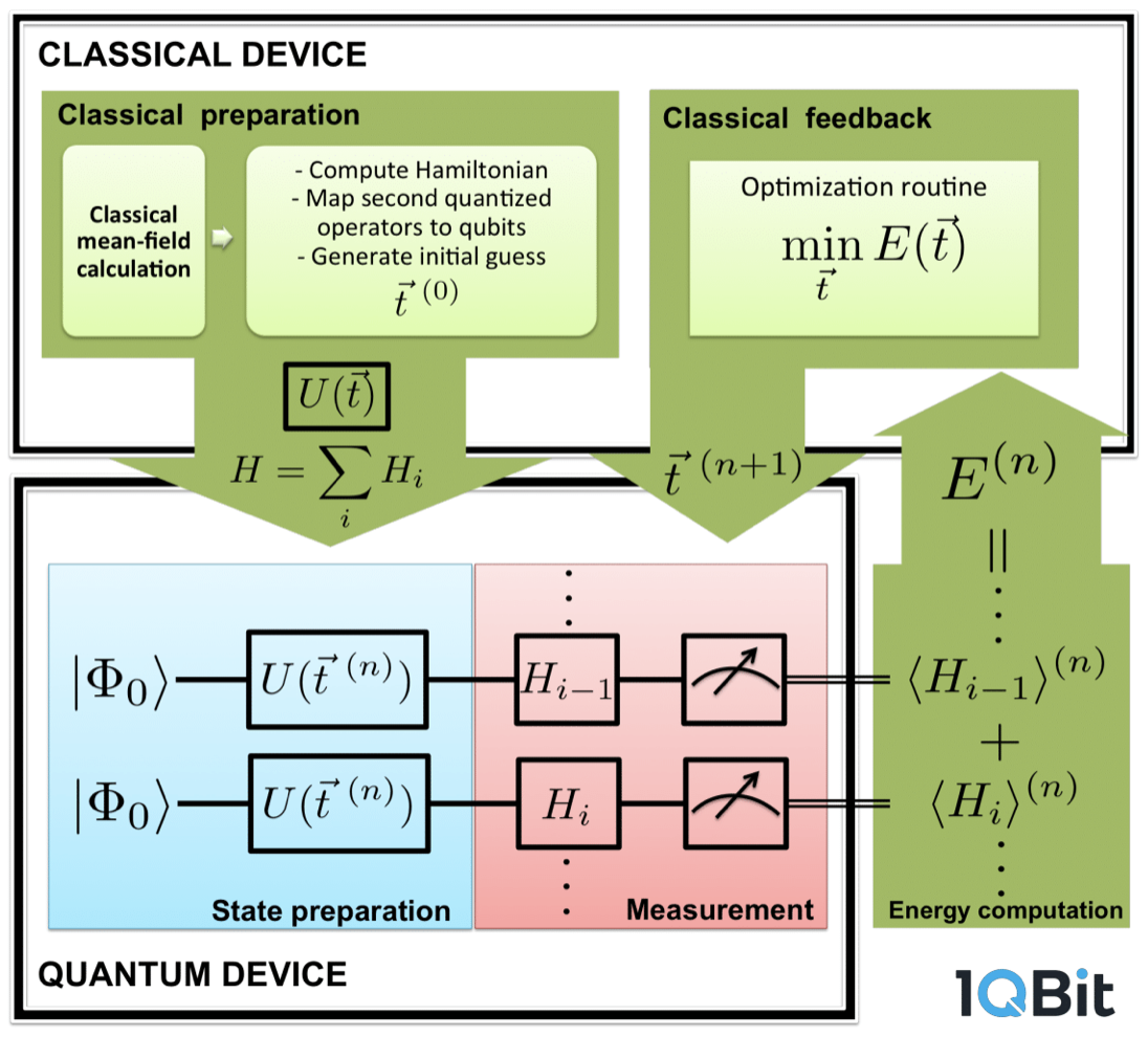 An illustration of how hybric quantum-classical algorithms work. Yanked from 1Qbit’s slides.
The hybrid approach has been successfully applied to modelling small atoms. It is also capable of finding solutions to some NP-complete problems (e.g., max-cut), though no one would give me an estimate of the runtime for this, not even in terms of the number of optimization steps.
Adiabatic quantum computers
Sometimes also called quantum annealers, these are, theoretically, suited to solving optimization problems where the optimization landscape has many local minima. But they don’t use logic gates to do this. The best analogy to a classical computer is that it’s an analog computer.
But let’s not be too down on the adiabatic quantum computer – up until not that long ago, there were a few applications that digital computers were too slow to handle, and only analog computers could do. And, at least one person thinks we should bring analog computers back.
Quantum supremacy
The immediate goal for a lot of quantum computing researchers is to demonstrate quantum supremacy: one single example of a real life problem being solved on a quantum computer faster than on the best classical computer. (Rigetti is currently offering a $1M prize for this, by the way.)
This has not been achieved yet, despite certain past claims by the Company-That-Shall-Not-Be-Named that it has done so.
Update: 8 months later, Google researchers claimed to have demonstrated quantum supremacy! To be clear, in this post, I was referring to D-Wave, which has a history of exaggerating its computers’ capabilities.
The industry presenters at this workshop were very optimistic that the hybrid quantum-classical approach has the potential to demonstrate quantum supremacy in the near future.
Some questions
Aside from the technical questions (e.g. how the hell do you express some arbitrary cost function as a Hamiltonian), I was left with the following burning questions about quantum computing in general.
Quantum computers as hardware accelerators?
We spent a lot of time on hybrid quantum-classical algorithms using NISQ. This is fair, since that’s the only current application of quantum computing.
But I couldn’t shake the feeling that in the hybrid model, the quantum computer is just acting as a glorified hardware accelerator to apply a specific Hamiltonian quickly. And, indeed, Fujitsu recently released a digital annealer, inspired by the adiabatic quantum computer.
If quantum supremacy were to be demonstrated by a hybrid quantum-classical algorithm beating out a classical computer, what would that really mean? Is it fair to compare specialized hardware against generalized hardware?
This makes me sound like I’m against hybrid algorithms, but that’s not true. They are the best way to use what we have right now, and it is never too early to look for applications.
What about all the other parts of a computer?
Speaking of generalized hardware, a classical computer is made up of rather a lot more than just the bits that do the calculation. What would those other parts of a quantum computer look like?
A classical computer without storage, memory, registers, and pipelines would be dramatically different. It’s hard to imagine that it would be anywhere near as powerful. Yet it’s unclear what these might even begin to look like in a quantum computer, which doesn’t allow reading or copying of qubits.
Maybe the end game quantum computer will find clever solutions to implement these things. Or maybe it won’t, and it will just be these limited, circuit-based models. Or maybe the end game quantum computer will have a form we can’t even begin to imagine right now. Personally, I’m hoping for option 3, but I don’t expect that it will happen terribly soon.
Summary
This “summary” turned out to be about 10 times longer than I had originally intended. If you read the whole thing, I’d love to buy you a coffee and hear your thoughts.
Here is a summary of the summary:
-
Quantum computing has really powerful operations that would require exponential time and space to do on a classical computer, but can be done polynomially on a quantum computer. The challenging part is making those really powerful operations result in a useful measurement.
-
Current quantum computers are small, have high error, and have so far failed to demonstrate any advantage. But, it is theoretically possible to have a fault-tolerant quantum computer.
-
We have a few examples of quantum algorithms with a proven advantage over classical algorithms. Broadly speaking, we’re not entirely sure what quantum computers can solve. It most likely can’t solve NP problems in P time, though.
-
Near term applications for quantum computing seem limited to some optimization problems, and we’re probably going to be stuck with hybrid quantum-classical approaches for a while.
-
There are a lot of challenges to building a “final form” quantum computer, not the least of which is that we don’t really know what it will look like yet.
Answers to the questions
I came to this workshop with some questions. After 4 days, I think I can make an attempt at some answers:
-
What is quantum computing and why is it so powerful? tl;dr: many degrees of freedom, powerful (but only linear) operations that would take ~\(2^n\) time on a classical computer.
-
What is the current state of the art in quantum computing? tl;dr: small, error prone, still looking for applications.
-
How could quantum computing impact my future career as a software engineer, and on what time scale? It would require breakthroughs in both technology and applicability before classical computing is seriously impacted. So, it probably won’t impact classical software engineers for a long time aside from researchers and those who work in scientific or high security fields.
a. When should I throw away my RSA keys? This question is difficult due to its specificity. Rather than give a timeline estimate, here are the milestones I’ll be looking for, to indicate that modern encryption might be in imminent danger:
- Someone demonstrates a fully error corrected qubit that survives long sequences of operations
- Someone connects multiple fault tolerant qubits, and all of them together survive long sequences of operations without decohering
- Someone demonstrates factorizing something small, say, the product of two single digit primes
Probably somewhere around stage 2, we’ll start seeing effort ramping up to guard against the arrival of the large scale fault tolerant quantum computer.
It’s also worth noting that all of this ado about encryption is due to one algorithm. If someone were to propose another game-changing algorithm, that would basically double the game-changing potential of quantum computing. I guess what I’m saying is, don’t take my prediction too seriously, it is very vulnerable to black swans.
-
Might I ever be interested in researching quantum computing? I mean, never say never, right? But currently, my interest remains casual. That said, there seems to be so much room for researchers, such as:
- electrical engineers and device physicists to make better qubits
- mathematicians and theoretical computer scientists to explore the algorithmic possibilities
- computer engineers with excellent imaginations to invent heretofore unseen architectures
- computational physicists and chemists to find near-term applications
-
If you’re very determined, you could prepare the same state and measure it many times, using the results to estimate the probability distributions. But this would probably kill any computational advantage of quantum computers, and you still wouldn’t get the true coefficients – you’d only get their squared amplitudes. ↩
-
Unless P = NP, but then classical computers can also solve NP problems in P time, so who cares about quantum computers at all? ↩
-
This claim was made by one of the presenters. I can’t find any other sources for it. Intuitively, this should depend on how many bits your RSA key has, no? Would love to see a source that really breaks this claim down. ↩